Oedometer test: one-dimensional consolidation (ASTM D2435)

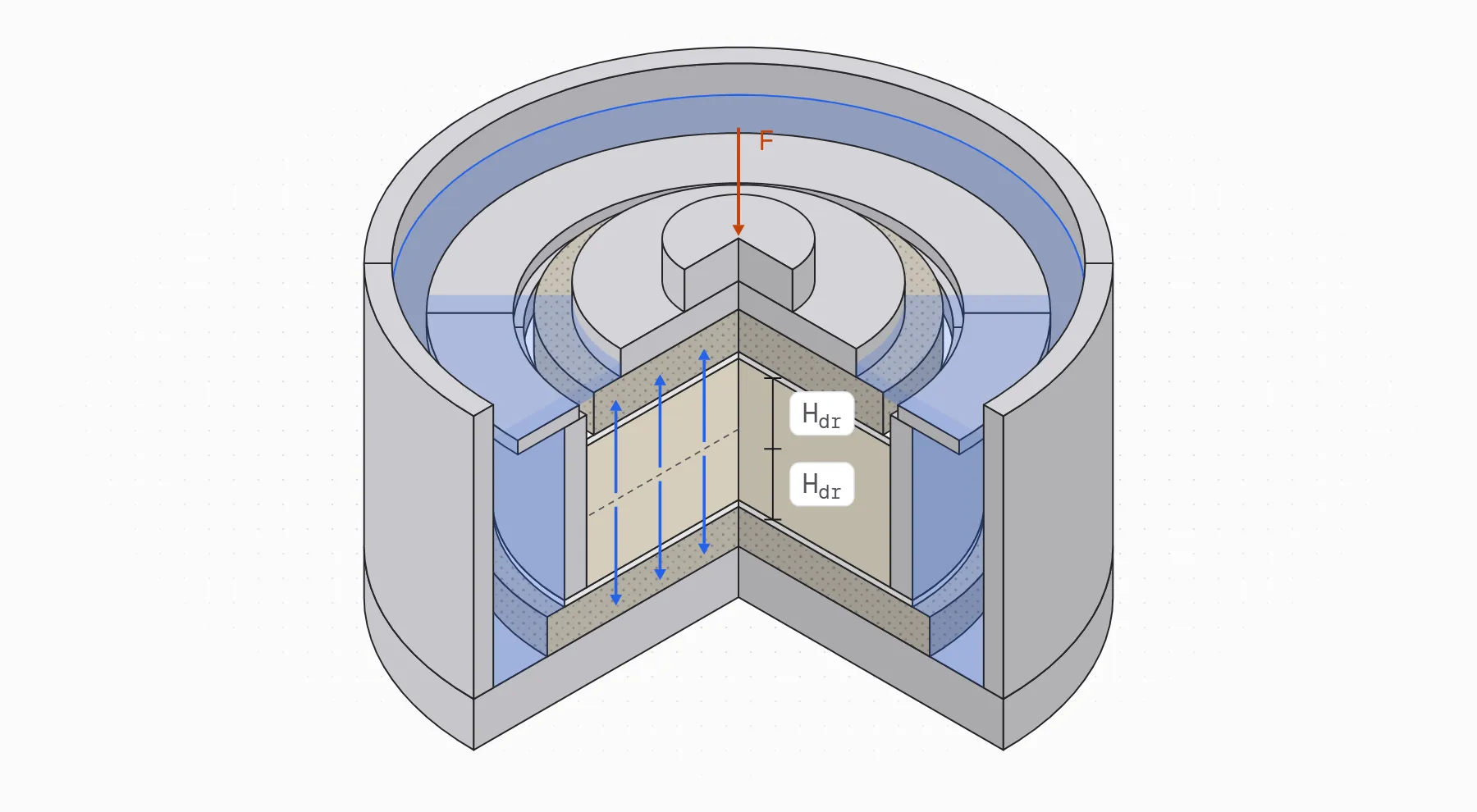
The oedometer test, also called the one-dimensional consolidation test, measures how much a saturated soil compresses under load and how fast. A specimen held in a rigid ring, so it can’t deform sideways, takes vertical load in increments while water drains through porous stones at its top and bottom, and you record its height over time. ASTM D2435 standardizes the procedure for incremental loading. The results give the parameters for computing consolidation settlement and its timing: the preconsolidation stress $\sigma'_p$, the compression index $C_c$, the recompression index $C_r$, the coefficient of consolidation $c_v$, the coefficient of volume change $m_v$ and the hydraulic conductivity $k_v$.

What consolidation is

Consolidation is the gradual compression of a saturated soil as water drains from its pores. When a load is applied, the pore water carries it at first as excess pore pressure. As water flows out, that pressure dissipates and the load passes to the soil skeleton as effective stress. The soil’s volume drops at the rate the water can leave, so in clays the process can take months or years in the field and minutes to hours in a specimen a couple of centimeters thick.

Karl Terzaghi formulated the theory in 1925 as a one-dimensional differential equation for how excess pore pressure changes with time and depth. It assumes a saturated, homogeneous soil, vertical flow and one-dimensional strain, and constant soil properties over each load increment. The oedometer test reproduces those conditions: the ring prevents lateral strain and the stones let the water drain vertically.

The coefficient of consolidation ties permeability and compressibility together:

$$c_v = \frac{k_v}{m_v \, \gamma_w} \qquad T_v = \frac{c_v \, t}{H_{dr}^2}$$

Where:

• $c_v$: coefficient of consolidation (m²/s)
• $k_v$: vertical hydraulic conductivity (m/s)
• $m_v$: coefficient of volume change (kPa⁻¹)
• $\gamma_w$: unit weight of water (kN/m³)
• $T_v$: time factor (dimensionless)
• $t$: elapsed time since the load was applied (s)
• $H_{dr}$: drainage path length, the longest distance water travels to a drainage boundary (m)

Because $t$ grows with $H_{dr}^2$, a 2 cm specimen draining from both faces finishes in minutes or hours, while a clay layer several meters thick takes years.

What the consolidation test gives you

The consolidation test measures two things for each load increment: the final compression and the time it takes. Plotting void ratio against the logarithm of effective stress gives the compression curve (the $e$-$\log \sigma'$ curve). It has a flat recompression branch, a bend near the preconsolidation stress and a steep straight virgin compression branch. Plotting compression against time within each increment gives the time curves, from which $c_v$ comes.

• Preconsolidation stress ($\sigma'_p$): the largest effective stress the soil has carried. Below it the soil is stiff; above it, it compresses along the virgin line. Comparing it with the current vertical effective stress gives the overconsolidation ratio, $OCR = \sigma'_p/\sigma'_{v0}$.
• Compression index ($C_c$): the slope of the virgin compression line on the $e$-$\log \sigma'$ plot.
• Recompression index ($C_r$): the slope on reloading below $\sigma'_p$, best measured on an unload-reload loop.
• Coefficient of consolidation ($c_v$): the rate of primary consolidation, from the time curve of each increment.
• Coefficient of volume change ($m_v$) and hydraulic conductivity ($k_v$): the strain per unit of stress, and the permeability that $c_v$ and $m_v$ imply.
• Coefficient of secondary compression ($C_\alpha$): the creep rate after primary consolidation ends.

For a normally consolidated clay layer of thickness $H_0$, the primary consolidation settlement under an increase from $\sigma'_{v0}$ to $\sigma'_f$ is

$$S_c = \frac{C_c \, H_0}{1 + e_0} \log_{10} \frac{\sigma'_f}{\sigma'_{v0}}$$

Where:

• $S_c$: primary consolidation settlement (m)
• $H_0$: initial thickness of the clay layer (m)
• $e_0$: initial void ratio of the layer
• $\sigma'_{v0}$, $\sigma'_f$: initial and final vertical effective stress at the middle of the layer (kPa)

For an overconsolidated clay, $C_r$ applies up to $\sigma'_p$ and $C_c$ beyond it. Our guide to foundation settlement works through these calculations.

Equipment

• Consolidometer (oedometer cell): a rigid base, a consolidation ring that confines the specimen laterally, porous stones at the top and bottom, a rigid top cap, and a bath that keeps the specimen submerged. The ring can be fixed (the specimen drains at top and bottom, but compresses only from the top) or floating (it compresses from both faces, with less side friction). USACE recommends an inside ring diameter of at least 2¾ in (70 mm), preferably 4 in, because a larger ring loses a smaller share of the load to side friction.
• Porous stones more pervious than the soil, cleaned after every test by boiling or in an ultrasonic bath.
• Loading device: a lever arm with weights, a pneumatic system or an automated load frame. It must apply each load quickly without impact and hold it constant for at least 24 h.
• Deformation indicator: a dial gauge or a linear displacement transducer (LVDT, linear variable differential transformer, or LST, linear strain transducer) that reads to 0.0001 in (about 0.0025 mm).
• Data acquisition system, if the frame and transducer are electronic.
• Trimming tools: trimming turntable, wire saw, knives or spatulas, a straightedge, and a recess tool to lower the soil surface inside the ring.
• Balance readable to 0.01 g.
• Vernier or digital calipers.
• Filter paper or filter disks, cut to the diameter of the specimen or slightly smaller.
• Distilled or demineralized water.
• Timer, and a thermometer for the bath.
• Equipment for water content (ASTM D2216) and for the specific gravity of solids (ASTM D854).

Oedometer test procedure (ASTM D2435)

The procedure below follows ASTM D2435 with an automated load frame and data acquisition. It is a wet setup, and the note at the end of the assembly covers the changes for a dry setup.

Methods A and B

ASTM D2435 has two methods, and they differ in how long each load stays on and on which increments you record deformation against time.

• Method A: each increment stays on for 24 h, or a multiple of 24 h. You record time and deformation on at least two increments. The result is the compression curve at 24 h, which mixes primary consolidation and secondary compression.
• Method B: you record time and deformation on every increment. The next increment goes on once primary consolidation has ended, judged with the log-time or root-time construction, or on Method A’s fixed schedule. Because you know where primary ends, you can separate it from secondary compression and get $c_v$ for every increment.

The procedure below is Method B, which an automated frame handles easily. For Method A, keep each load on for 24 h and record time curves on at least two increments.

Load schedule

The agency requesting the test sets the loads, including whether there is an unload-reload cycle. D2435’s traditional schedule doubles the stress at each increment, a load increment ratio $LIR = \Delta\sigma/\sigma = 1$. Near the expected preconsolidation stress, smaller steps define $\sigma'_p$ better: USACE suggests multiplying the load by 1.5 or 1.25 there. Very small steps produce little compression, so the end of primary can become hard to see. When unloading, each step removes between half and three quarters of the stress ($LIR$ from −0.50 to −0.75).

The maximum load should go well past $\sigma'_p$, about four times the expected value according to FHWA, so the virgin line is straight and well defined. An example schedule in kPa: seating, 12.5, 25, 50, 100, 200, 400, 800, 400, 200, 400, 800, 1600, 800, 400, 100, seating.

Equipment preparation

1. Grease the specimen ring and the cutting shoe (if it isn’t built into the ring).
2. Weigh the greased ring together with one filter disk. Record this mass as $M_{rf}$.
3. Measure the diameter ($D_r$) and the height ($H_r$) of the ring.
4. Boil the porous stones or clean them ultrasonically, then store them in water.
5. Measure how far the recess tool goes into the ring ($H_{rt}$).
6. Measure the thickness of one filter disk ($H_{fd}$).
7. Weigh the top cap, the top stone and the moment break together ($M_{tc}$).
8. Calibrate the apparatus compressibility. Assemble the cell with its stones and wet filters and no soil, apply the same loads you’ll use in the test, read the deformation under each, then unload in the same order. These readings give the apparatus compression for each load, which you subtract from the specimen’s deformation. In stiff or sandy soils this correction can be a large share of what you measure.

Specimen preparation

Disturbance is the main source of error in this test, so trim the specimen in a humid room and handle it as little as possible.

1. Trim the specimen into the cutting ring, keeping its vertical orientation. On a trimming turntable, rough-cut the soil a little larger than the ring and shave it down as the ring advances, so the soil fills the ring with no gaps.
2. Recess the soil surface inside the ring to leave room for the top filter disk. Use the recess tool on the top, and trim the excess off the bottom with a wire saw. With a floating ring, recess both the top and the bottom.
3. Weigh the specimen with the ring and the filter. Record this value as $M_{srf,i}$.
4. Keep the trimmings for water content and, if the soil’s $G_s$ isn’t known, for a specific gravity test.

Assembly (wet method)

1. Fill the base of the oedometer with water.
2. Place the bottom stone and the filter, both already wetted.
3. Blot the excess water off the stone with paper.
4. Set the ring with the specimen on top of the stone.
5. Fit a gasket around the ring.
6. Place the clamping collar to hold it in place.
7. Blot the top stone with paper and place it on the specimen (the filter goes on first).
8. Place the top cap on the stone.
9. Move the whole assembly to the load frame. Install the displacement transducer and the loading arm. Measure and record the tare force of the assembly ($F_{tr}$).
10. Apply a small seating load (about 5 N), set the transducer near the start of its range so it can also measure swelling, and record the initial reading ($V_{disp,0}$) and the input voltage ($V_{in,0}$).

Note: In a dry setup, the cell is assembled without water: skip steps 1 and 3, place the bottom stone and the filter dry in step 2, and in step 7 place the top stone without blotting it.

Loading and readings

1. Depending on the software, save the data in a single file or in one file per load, and check that the equipment clock is synchronized with the data acquisition system.
2. Start logging data every second. Write down the time, the applied load ($F_j$), the initial displacement reading ($V_{disp,j,0}$) and the file name. Apply the first increment.
3. Fill the water bath about 1 minute after applying the first increment. If the soil swells, add load quickly until the swelling stops: a specimen that swells gives a rounder compression curve and a poorly defined $\sigma'_p$.
4. For each load, record displacement against time. The first seconds define the start of consolidation, so start recording just before you touch the equipment, then reduce the reading frequency so you don’t generate too much data. With a manual dial gauge, readings at 0.1, 0.2, 0.5, 1, 2, 4, 8, 15 and 30 min and at 1, 2, 4, 8 and 24 h are usually enough.
5. Keep the bath temperature steady. USACE asks that it vary no more than ±2 °C during the test.
6. During each increment, plot the readings against $\sqrt{t}$ and against $\log t$. In a teaching lab, do both for at least one increment.
7. Apply the next load once primary consolidation has ended according to those constructions (Method B), or after 24 h (Method A).
8. After passing $\sigma'_p$, run the unload-reload cycle of the schedule. Before removing each unloading step, wait until the rebound stops changing with time.
9. At the maximum load, leave the load on for one log cycle of time past the end of primary consolidation so you can measure secondary compression.

Unloading and final measurements

1. At the end of the test, unload to the seating load, keep the transducer in place and let the specimen swell until the readings stop changing. A small final load limits swelling and the error it causes in the final water content.
2. Record the final displacement reading ($V_{disp,f}$).
3. Take the apparatus out of the load frame and drain the water bath.
4. Remove the top cap and the top stone.
5. Scrape off the soil that extruded past the ring and oven-dry it. Record that mass as $M_{extr}$. If you used a floating ring, repeat for the bottom.
6. Blot the specimen surface dry and weigh the ring, specimen and filter again ($M_{srf,f}$).
7. For a teaching lab, measure the final height of the specimen plus one filter ($H_{f,g}$) with a dial gauge.
8. Take the specimen out of the ring and remove the filter.
9. Weigh the wet specimen ($M_{t,f}$).
10. If you are going to run index tests, take a wedge-shaped portion to measure the final water content ($\omega_f$).
11. Otherwise, oven-dry the entire specimen and record its dry mass ($M_{ds}$).
12. Collect and dry any material left on the filter or the ring. Record it as $M_{dw}$.

Calculations

Initial state of the specimen

1. Dry mass of the specimen ($M_d$), from either of the following expressions:

$$M_d = M_{ds} + M_{dw} + M_{extr}$$

or:

$$M_d = \frac{M_{t,f}}{1 + \frac{\omega_f}{100}}$$

Where:

• $M_d$: total dry mass of the specimen (g)
• $M_{ds}$: dry mass, not including the extruded material or the washings (g)
• $M_{dw}$: dry mass of the washings (g)
• $M_{extr}$: dry mass of the extruded material (g)
• $M_{t,f}$: final wet mass of the specimen (g)
• $\omega_f$: final water content of the specimen (%)

2. Initial water content ($\omega_N$):

$$\omega_N = \left( \frac{M_{srf,i} - M_{rf}}{M_d} - 1 \right) \times 100$$

Where:

• $\omega_N$: natural water content of the specimen (%)
• $M_{srf,i}$: initial mass of the specimen, ring and filter together (g)
• $M_{rf}$: mass of the ring with the filter (g)

3. Initial height of the specimen ($H_i$), to the nearest 0.01 mm. ASTM D2435 allows two ways. You can measure it: average at least four evenly spaced readings over the top (and bottom) surface of the specimen with a dial comparator, and subtract the thickness of any filter included in the reading. Or you can calculate it from the ring:

$$H_i = H_r - H_{rt} - H_{fd}$$

Where:

• $H_i$: initial height of the specimen (cm)
• $H_r$: height of the specimen ring (cm)
• $H_{rt}$: thickness of the recess spacer, how far the recess tool reaches into the ring (cm)
• $H_{fd}$: thickness of the filter that sits inside the ring with the specimen (cm)

The standard subtracts each of them only when it applies: without a recess, $H_{rt} = 0$, and without a filter inside the ring, $H_{fd} = 0$.

4. Initial void ratio ($e_i$). The volume of solids is $M_d/(G_s \rho_w)$, so:

$$e_i = \left( \frac{\pi}{4} D_r^2 H_i G_s \rho_w \right) \frac{1}{M_d} - 1$$

Where:

• $e_i$: initial void ratio
• $D_r$: diameter of the specimen ring (cm)
• $H_i$: initial height of the specimen (cm)
• $\rho_w$: density of water (g/cm³)
• $G_s$: specific gravity of the solids (dimensionless)
• $M_d$: dry mass of the specimen (g)

5. Initial degree of saturation ($S_i$):

$$S_i = \frac{G_s \cdot \omega_N}{e_i}$$

Where:

• $S_i$: initial degree of saturation (%)
• $G_s$: specific gravity of the solids
• $\omega_N$: natural water content (%)
• $e_i$: initial void ratio

The time analysis assumes a saturated specimen. If $S_i$ comes out well below 100%, treat $c_v$ with caution. The phase relations lesson covers these relationships in detail.

Applied stress

6. Effective stress applied in each increment $j$ ($\sigma'_{a,j}$):

$$\sigma'_{a,j} = \left( \frac{F_j - F_{tr} + \frac{M_{tc} \cdot g}{1000}}{A} \right) \times 10$$

Where:

• $\sigma'_{a,j}$: effective stress applied in increment $j$ (kPa)
• $F_j$: force read by the load system in increment $j$ (N)
• $F_{tr}$: tare force of the system (N)
• $M_{tc}$: mass of the top cap, the top stone and the moment break (g)
• $g$: acceleration due to gravity (m/s²)
• $A$: area of the specimen, $\pi D_r^2/4$ (cm²)

ASTM D2435 defines the stress as the total axial load on the specimen divided by its area. That load has two parts. The load system applies $F_j - F_{tr}$, its reading minus the tare of the parts installed with it. The top cap, the top stone and the moment break sit on the specimen below the point where the force is measured, so their weight $M_{tc} \cdot g$ also bears on the soil but never shows in $F_j$. It is added, as in Germaine’s consolidation procedure for MIT, where the stress is the applied load minus the tare load plus the top cap and stone, over the area. The factor 1000 turns grams into kilograms, and the factor 10 turns N/cm² into kPa. With the top cap’s weight subtracted, every stress would be low by twice that weight, which matters most in the first increments.

The stress is effective once primary consolidation ends, when the excess pore pressure has dissipated. Friction between the soil and the ring is not considered here. USACE reports that more than 20% of the load can be lost to side friction in a fixed ring, and about half that in a floating ring. To include it, subtract the force lost to friction from $F_j$.

Deformation and strain

7. Converting voltages to displacements ($\delta_{j,i}$):

$$\delta_{j,i} = \left( \frac{V_{disp,j,i}}{V_{in,j,i}} - \frac{V_{disp,0}}{V_{in,0}} \right) \cdot CF_{disp}$$

Where:

• $\delta_{j,i}$: displacement at reading $i$ during increment $j$ (cm)
• $V_{disp,j,i}$: transducer output voltage at reading $i$ (V)
• $V_{in,j,i}$: input voltage at reading $i$ (V)
• $V_{disp,0}$: initial output voltage (V)
• $V_{in,0}$: initial input voltage (V)
• $CF_{disp}$: transducer calibration factor (cm/V/Vin)

8. Deformation of the specimen at reading $i$ of increment $j$ ($\Delta H_{j,i}$), with the apparatus compression removed:

$$\Delta H_{j,i} = \delta_{j,0} - \delta_{j,i} - \Delta H_{m,j}$$

Where:

• $\Delta H_{j,i}$: change in height of the specimen in increment $j$, reading $i$ (cm)
• $\delta_{j,0}$: displacement at the start of increment $j$ (cm)
• $\Delta H_{m,j}$: compression of the apparatus for the step to load $j$, from the calibration (cm)

9. Axial strain at reading $i$ ($\varepsilon_{a,j,i}$), accumulated from the start of the test:

$$\varepsilon_{a,j,i} = \varepsilon_{s,j} + \left( \frac{\Delta H_{j,i}}{H_i} \right) \times 100$$

Where:

• $\varepsilon_{a,j,i}$: axial strain at reading $i$ of increment $j$ (%)
• $\varepsilon_{s,j}$: strain at the start of increment $j$, equal to the strain at the end of increment $j-1$ (%); for the first increment, $\varepsilon_{s,1} = 0$
• $H_i$: initial height of the specimen (cm)

Coefficient of consolidation: log-time and root-time methods

10. ASTM D2435 uses two graphical constructions on the time curve of each increment. Both give a time for a known degree of consolidation, and $c_v$ follows from Terzaghi’s theory.

Casagrande’s log-time method:

1. Plot the deformation or strain against the logarithm of time.
2. Find the corrected zero, $d_0$, which a log scale can’t show directly. Take a time $t_1$ in the early, curved part and the time $4t_1$. Find the vertical difference between their readings and mark $d_0$ that same distance above the reading at $t_1$.
3. Find the end of primary consolidation, $d_{100}$: the intersection of the tangent at the steepest part of the curve with the straight line of the final, secondary compression part.
4. The midpoint $d_{50} = (d_0 + d_{100})/2$ gives $t_{50}$ on the curve.

$$c_v = \frac{T_{50} \, H_{dr}^2}{t_{50}}, \qquad T_{50} = 0.197$$

Taylor’s root-time method:

1. Plot the deformation or strain against the square root of time.
2. Draw a straight line through the initial straight part of the curve and extend it back to $t = 0$ to get the corrected zero, $d_0$.
3. From $d_0$, draw a second line whose abscissas are 1.15 times those of the first.
4. The point where this second line cuts the curve gives $d_{90}$ and $\sqrt{t_{90}}$. The end of primary is $d_{100} = d_0 + (d_{90} - d_0)/0.9$.

$$c_v = \frac{T_{90} \, H_{dr}^2}{t_{90}}, \qquad T_{90} = 0.848$$

Where:

• $c_v$: coefficient of consolidation (cm²/s; multiply by $10^{-4}$ for m²/s)
• $T_{50}$, $T_{90}$: time factors for 50% and 90% average consolidation
• $t_{50}$, $t_{90}$: times to reach 50% and 90% of primary consolidation (s)
• $H_{dr}$: drainage path, half the specimen height at 50% consolidation when both faces drain, $H_{dr} = H_i (1 - \varepsilon_{50}/100)/2$ (cm)
• $\varepsilon_{50}$: strain at 50% consolidation (%)

The root-time method only needs the curve up to $t_{90}$, so it suits increments that you want to end as soon as primary consolidation does. The log-time method needs the curve well past $t_{100}$, but it also gives the secondary compression slope. The two rarely agree exactly. Report both, or their average, and plot $c_v$ against $\log \sigma'_a$ at the average stress of each increment.

Compression curve and compression index

11. Void ratio at the end of primary consolidation of each increment ($e_j$):

$$e_j = e_i - \frac{\varepsilon_{100,j}}{100} \, (1 + e_i)$$

Where:

• $e_j$: void ratio at the end of primary consolidation in increment $j$
• $\varepsilon_{100,j}$: strain at the end of primary consolidation in increment $j$ (%)

Plot $e_j$ (or $\varepsilon_{100,j}$) against $\sigma'_{a,j}$ on a log scale to get the compression curve. With Method A, the points are the end-of-increment values at 24 h.

12. Compression index ($C_c$) and recompression index ($C_r$):

$$C_c = \frac{e_1 - e_2}{\log_{10} \sigma'_2 - \log_{10} \sigma'_1}$$

Where:

• $C_c$: compression index (dimensionless)
• $\sigma'_1$, $\sigma'_2$: two stresses on the straight virgin compression line (kPa)
• $e_1$, $e_2$: the void ratios at those stresses

If you choose $\sigma'_2 = 10\,\sigma'_1$, the denominator is 1 and $C_c$ is the drop in void ratio over one log cycle. The recompression index $C_r$ is the same slope measured on the unload-reload loop. The first loading branch is less reliable for $C_r$ because disturbance makes it steeper than the soil in the ground.

On a strain plot, the same slopes are the compression ratio $CR = C_c/(1 + e_i)$, the recompression ratio $RR = C_r/(1 + e_i)$ and the swelling ratio $SR$, the slope on unloading.

Preconsolidation stress: Casagrande construction

13. Preconsolidation stress ($\sigma'_p$) with Casagrande’s construction.

On the $e$-$\log \sigma'$ curve (or the $\varepsilon$-$\log \sigma'$ curve):

1. Draw the tangent to the steepest part of the curve, on the virgin compression line.
2. Find the point of maximum curvature, where the slope changes from flat to steep, and draw a horizontal line through it.
3. Draw the tangent to the curve at that same point.
4. Draw the bisector of the angle between the horizontal line and that tangent.
5. The stress where the bisector meets the virgin line tangent from step 1 is $\sigma'_p$.

Step 2 depends on judgment. When the point of maximum curvature isn’t clear, try several and report the range.

The strain energy method gives a second estimate on an arithmetic scale. Compute the work of each increment:

$$\Delta W_j = \frac{\sigma'_{a,j-1} + \sigma'_{a,j}}{2} \cdot \frac{\varepsilon_{100,j} - \varepsilon_{100,j-1}}{100}$$

Where:

• $\Delta W_j$: work per unit volume in increment $j$ (kJ/m³ with stresses in kPa)

Plot the cumulative work against $\sigma'_a$. The points form two straight trends, one at low stress and one at high stress, and $\sigma'_p$ is the stress where they cross.

Coefficient of volume change and hydraulic conductivity

14. Coefficient of volume change ($m_{v,j}$):

$$m_{v,j} = \frac{\varepsilon_{100,j} - \varepsilon_{100,j-1}}{\sigma'_{a,j} - \sigma'_{a,j-1}} \cdot \frac{1}{100}$$

Where:

• $m_{v,j}$: coefficient of volume change (kPa⁻¹)
• $\varepsilon_{100,j}$: strain at the end of primary consolidation in increment $j$ (%)
• $\varepsilon_{100,j-1}$: strain at the end of primary consolidation in the previous increment (%)
• $\sigma'_{a,j}$ and $\sigma'_{a,j-1}$: effective stresses of increments $j$ and $j-1$ (kPa)

15. Hydraulic conductivity ($k_{v,j}$), from $k_v = c_v \, m_v \, \gamma_w$ with the strain measured within the increment:

$$k_{v,j} = c_{v,j} \cdot \gamma_w \cdot \frac{\varepsilon_{100,j} - \varepsilon_{s,j}}{\sigma'_{a,j} - \sigma'_{a,j-1}} \cdot \frac{1}{100}$$

Where:

• $k_{v,j}$: hydraulic conductivity for increment $j$ (m/s)
• $c_{v,j}$: coefficient of consolidation (m²/s)
• $\gamma_w$: unit weight of water, $\gamma_w = \rho_w \cdot g$ (kN/m³)
• $\varepsilon_{100,j}$: strain at the end of primary consolidation (%)
• $\varepsilon_{s,j}$: strain at the start of increment $j$ (%)
• $\sigma'_{a,j}$ and $\sigma'_{a,j-1}$: effective stresses (kPa)

This $k_v$ is an indirect estimate from consolidation theory. A permeability test measures it directly.

Secondary compression

16. Coefficient of secondary compression ($C_{\alpha\varepsilon}$), from the straight part of the time curve after the end of primary consolidation:

$$C_{\alpha\varepsilon} = \frac{\varepsilon_{t_2} - \varepsilon_{t_1}}{100 \, \log_{10} (t_2 / t_1)}$$

Where:

• $C_{\alpha\varepsilon}$: coefficient of secondary compression in strain (dimensionless); multiplied by $(1 + e_i)$ it gives $C_\alpha$ in terms of void ratio
• $t_1$, $t_2$: two times after the end of primary consolidation, $t_p$ (s)
• $\varepsilon_{t_1}$, $\varepsilon_{t_2}$: strains at those times (%)

Final height and height check

17. Final height of the specimen ($H_f$):

$$H_f = H_{f,g} - H_{fd}$$

Where:

• $H_f$: final height of the specimen (cm)
• $H_{f,g}$: final height measured with the dial gauge (including one filter) (cm)
• $H_{fd}$: thickness of the filter (cm)

18. Height error ($E_H$):

$$E_H = \left( \frac{H_i - H_f - \Delta H_f}{H_i} \right) \times 100$$

Where:

• $E_H$: error in the height calculation (%)
• $H_i$: initial height of the specimen (cm)
• $H_f$: final height of the specimen (cm)
• $\Delta H_f$: total deformation calculated over the test (cm)

Report

Include the following in the report:

1. The method used (A or B), the load schedule and the duration of each increment.
2. Plots of deformation versus the square root of time and versus the logarithm of time for each load step, with the interpretation constructions drawn on them.
3. The apparatus compressibility curve.
4. The error associated with specimen extrusion.
5. The procedures and results of the error analysis on the height measurements.
6. A plot of strain versus applied effective stress $\sigma'_a$, on both logarithmic and arithmetic scales, clearly marking the end of primary consolidation and the end of each stage. Draw the lines carefully, especially where the loading direction changes.
7. A plot of strain energy (work done) versus $\sigma'_a$.
8. The preconsolidation stress from the Casagrande method and from the strain energy method. Show and label both values on the $\varepsilon$ vs. $\sigma'_a$ plot.
9. The compression index $C_c$, the recompression index $C_r$, and the ratios $CR$, $RR$ and $SR$, shown on the same plot.
10. A plot of $c_v$ versus $\log \sigma'_a$, using both the root $t$ and the $\log t$ methods, with each point placed at the average stress of its stage.
11. A plot of $\log k_v$ versus $\log \sigma'_a$ and also versus void ratio $e$, with the points placed at the average stress and void ratio of each increment.
12. A summary table for each load stage with: $\sigma'_a$, $e_{50}$, $\varepsilon_s$, $t_{50}$, $\varepsilon_{50}$, $t_{90}$, $t_p$, $\varepsilon_{100}$, $t_f$, $\varepsilon_f$, $c_v$, $m_v$, $k_v$, $C_{\alpha \varepsilon}$.
13. An overall summary table for the test, with $\sigma'_p$, $C_c$, $C_r$, $CR$, $RR$ and $SR$ and the initial state of the specimen (and final state, if $H_f$ was measured): water content, void ratio, degree of saturation and density.

Typical values

These ranges help you check whether a result is reasonable, and they don’t replace the test.

• Compression index: for clays of low to medium sensitivity, Terzaghi and Peck’s correlation estimates $C_c \approx 0.009\,(LL - 10)$, with the liquid limit $LL$ from the Atterberg limits in percent. Measured values can differ from these correlations by a wide margin.
• Recompression index: $C_r/C_c$ usually falls between 0.02 and 0.20, so $C_r$ is often about a tenth of $C_c$.
• Coefficient of consolidation: from about 1 m²/yr in clays of low permeability to 1000 m²/yr or more in sandy or fissured clays. Examples: Boston Blue Clay (CL) about 12 ± 6 m²/yr, San Francisco Bay Mud (CL) 0.6 to 1.2 m²/yr, Mexico City clay (MH) 0.3 to 0.5 m²/yr.
• Secondary compression: $C_\alpha/C_c$ is about 0.05 ± 0.01 in organic clays and silts and 0.075 ± 0.01 in peats.
• Stress history from the OCR: 1 is normally consolidated, 1 to 2 lightly overconsolidated, 2 to 8 moderately overconsolidated, and above 8 heavily overconsolidated.

Common mistakes

• Disturbance rounds off the bend in the compression curve, lowers $\sigma'_p$ and $C_c$, raises $C_r$ and lowers $c_v$ and $C_\alpha$. You can gauge it from the strain needed to reload the specimen to its in situ vertical stress: Terzaghi and coauthors rate a specimen A (the best) below 1%, B from 1 to 2%, and down to E above 8%, and soft clays should rate at least B.
• If the next load goes on before primary consolidation ends, $C_c$ comes out low and $c_v$ high.
• If the test barely passes $\sigma'_p$, the virgin line isn’t defined and both $\sigma'_p$ and $C_c$ come out low.
• $C_r$ taken from the first loading branch overestimates settlement in the overconsolidated range. Measure it on the unload-reload loop.
• A specimen that swells at low loads blurs $\sigma'_p$. Add load until the swelling stops, or flood the cell only once the specimen is on the virgin line.
• Without the apparatus compressibility correction, stiff soils look more compressible than they are.

References

• ASTM International. (2025). ASTM D2435/D2435M-25: Standard test methods for one-dimensional consolidation properties of soils using incremental loading. https://store.astm.org/d2435_d2435m-25.html
• U.S. Army Corps of Engineers. (1970, with changes through 1986). EM 1110-2-1906: Laboratory soils testing, Appendix VIII, Consolidation test.
• Loehr, J. E., Lutenegger, A., Rosenblad, B., & Boeckmann, A. (2016). Geotechnical site characterization (Geotechnical Engineering Circular No. 5, FHWA-NHI-16-072), chapter 6. Federal Highway Administration. https://www.fhwa.dot.gov/engineering/geotech/pubs/nhi16072.pdf
• Samtani, N. C., & Nowatzki, E. A. (2006). Soils and foundations reference manual, Volume I (FHWA-NHI-06-088), chapters 5 and 7. Federal Highway Administration. https://www.fhwa.dot.gov/engineering/geotech/pubs/nhi06088.pdf
• Germaine, J. T. (2004). Laboratory assignment 9: Consolidation test. 1.103 Civil Engineering Materials Laboratory, MIT OpenCourseWare. https://ocw.mit.edu/courses/1-103-civil-engineering-materials-laboratory-spring-2004/d3c36fbd5fecb45bd0a1230cb05aec75_lab_9.pdf
• Germaine, J. T., & Germaine, A. V. (2009). Geotechnical laboratory measurements for engineers. Wiley.
• Holtz, R. D., Kovacs, W. D., & Sheahan, T. C. (2011). An introduction to geotechnical engineering (2nd ed.). Pearson.