

Direct shear test (ASTM D3080): procedure and calculation
How to run the direct shear test per ASTM D3080 and calculate the shear strength of soil: Mohr-Coulomb envelope, cohesion and friction angle.
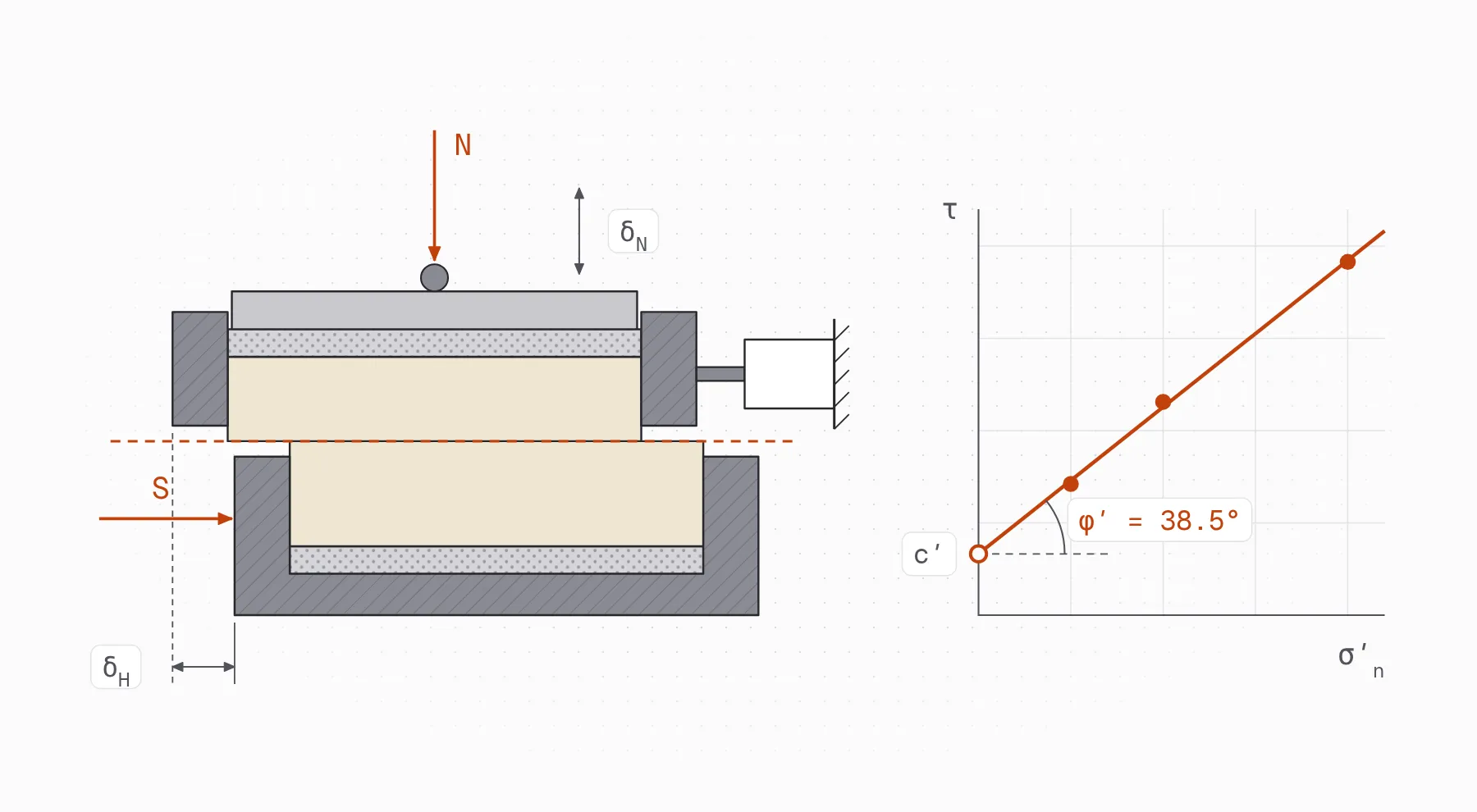
The direct shear test measures the shear strength of soil along a plane the apparatus imposes. A specimen sits in a box split into two halves; it is consolidated under a normal load, and then one half is pushed past the other at a slow, constant rate while the shear force and the displacements are recorded. ASTM D3080 covers the test under consolidated drained conditions, so the result is the soil’s drained (effective) strength. Run at three or more normal stresses, it gives the Mohr-Coulomb envelope: the effective cohesion and the friction angle that bearing capacity, earth pressure and slope stability calculations start from.
Direct shear calculator
Calculator · ASTM D3080
Trials
The standard asks for at least three different normal stresses: with two, the line always goes through both points and the angle doesn't come from the data.
| Trial | Normal stress(kg/cm²) | Shear stress(kg/cm²) |
|---|---|---|
| #1 | ||
| #2 | ||
| #3 |
With 3 trials at normal stresses from 0.50 to 2.00 kg/cm², the fitted line is τf = 0.332 + σ·0.796. It gives a friction angle of 38.5° and a cohesion of 0.332 kg/cm², with a fit of R² = 0.9983
Shear strength parameters
| Quantity | Value |
|---|---|
| Cohesion · cthe line's intercept | 0.332kg/cm² |
| Slope · tan φleast squares over the trials | 0.7957 |
| Friction angle · φatan of the slope | 38.51° |
| The line's fit · R²1 − SSres / SStot | 0.9983 |
This calculator is offered for information and technical support. It doesn't replace professional judgment or the reviews due, and its use is the user's responsibility.
The calculator also has a page of its own, to keep at hand: the direct shear calculator. The cohesion and friction angle it gives are what the bearing capacity and lateral earth pressure calculators take, and what a retaining wall design starts from.
What is the direct shear test?
The test forces the soil to fail on a horizontal plane at the joint between the two halves of the box. Each trial gives one pair of values at failure: the normal stress on that plane and the shear stress the soil resisted. Because drainage is allowed during consolidation and the shearing is slow, no excess pore pressure builds up, and the stresses measured are effective stresses.
ASTM D3080 describes the test of a single specimen; in practice three or more specimens of the same soil are sheared, each under a different normal load, and the envelope is drawn through their results. Interpreting that set of tests is outside the standard’s scope.
The test is quick and cheap, and the short drainage path lets pore pressures dissipate faster than in other drained tests. It also has limits worth knowing before you use its numbers:
- The failure plane is forced through the middle of the specimen, which may not be the soil’s weakest plane. This becomes an advantage when you want the strength along a known plane, such as a bedding plane or the contact between soil and a geosynthetic.
- Shear stress and displacement are not uniform inside the specimen, so no shear strain can be calculated. The test gives strength, not a stress-strain curve or a modulus.
- The contact area between the two halves shrinks as they slide apart. This adds uncertainty to the stresses, but it should not change the ratio between shear and normal stress.
- The equipment cannot run an undrained test. Shearing fast without controlling the specimen’s volume gives partial drainage and wrong strength parameters.
Shear strength of soil: the Mohr-Coulomb criterion
The shear strength of soil on a plane depends on the effective normal stress acting on it. The Mohr-Coulomb criterion idealizes that relationship as a straight line:
where:
- is the shear stress at failure on the plane (kPa),
- is the effective normal stress on the plane (kPa),
- is the effective cohesion, the line’s intercept (kPa),
- is the effective angle of internal friction, the line’s slope angle (°).
Cohesion and friction angle
In a direct shear test the failure plane is known, so each trial plots directly as a point and the envelope is the line through the points. Clean sand has practically no cohesion, so for sand the line passes close to the origin and the friction angle can be read from a single trial. For clays and silts the intercept depends on the stress history: a normally consolidated clay gives an envelope through the origin, while an overconsolidated or compacted soil shows an intercept.
Peak and ultimate strength
A dense sand reaches a peak shear force, then softens to a lower, roughly constant value as shearing continues. It also dilates: the top cap rises as the grains ride over each other. A loose sand shows no clear peak; its shear force climbs to a steady value while the specimen contracts. Both values matter, so read two points off each test:
- the peak shear force , the maximum reached;
- the ultimate shear force , the steady value at the end of shearing.
The ultimate value of a single pass is not the true residual strength of a clay. That takes very large displacements, and USACE measures it with a repeated direct shear test that reverses the box several times (EM 1110-2-1906, Appendix IXA).
Equipment
- Direct shear device with a motor that drives one half of the box at a constant rate, adjustable over a wide range so that slow drained tests are possible.
- Normal load system, with calibrated weights on a hanger or with pneumatic pressure, able to apply the load without impact and hold it constant for the whole test. Calibrate it so the load you read is the load the specimen gets.
- Shear box, square or circular, split horizontally into two halves held together by alignment screws, with gap screws to separate them before shearing. Inside go the porous stones or the grooved (ribbed) plates that grip the specimen and let it drain, and a loading cap on top.
- Counterbalance system, useful for tests at low normal loads.
- Load cell or proving ring to measure the shear force.
- Displacement transducers (LVDTs) or dial indicators for the horizontal and the vertical displacement. For reference, the USACE manual asks for a vertical indicator with a range of 0.25 in and an accuracy of 0.0001 in (about 0.0025 mm), and a horizontal one with a range of 0.5 in and an accuracy of 0.001 in (about 0.025 mm).
- Data acquisition system compatible with the sensors.
- Balances readable to 0.1 g and 0.01 g.
- Caliper or depth gauge to measure the box and the specimen.
- Timer, for the consolidation readings.
- For sand specimens: a tamper that fits the box, a pouring container, and a funnel with a tube to deposit the sand gently.
- For saturated or fine-grained soils: distilled water to keep the specimen submerged, and trimming tools to cut intact specimens to the size of the box.
Direct shear test procedure (ASTM D3080)
The steps below follow ASTM D3080 and the MIT dry sand laboratory this lesson is based on (Germaine, 2004). They apply to any shear device, with adjustments for its controls. The example is a set of six tests on dry quartz sand, loose and dense specimens, each density at three normal loads. The MIT lab uses masses of about 17.5, 27.5 and 47.5 kg acting on the specimen, counting the parts of the apparatus that rest on it.
For a project, pick the normal stresses from the field problem: the highest should be at least the largest normal stress expected in the field, so the envelope is never extrapolated.
1. Check the specimen size
The box limits the largest particle the specimen can hold. ASTM D3080 requires the specimen width (or diameter) to be at least 10 times the maximum particle size, and it also sets a minimum thickness tied to the maximum particle size and a minimum width-to-thickness ratio. Check those limits in the standard against your box before testing. Research on coarse materials finds that a ratio of 10 does not remove the effect of specimen size on the friction angle, and points to a width of about 60 times the largest particle (Deiminiat and Li, 2022). If the soil has particles that are too large, use a larger box or a triaxial test; with the 3 × 3 in box of the USACE manual, that applies to anything retained on the No. 4 sieve (4.75 mm).
2. Prepare the specimen
Dense specimens are tamped by hand to reach a high relative density. Loose specimens are deposited through a funnel so the grains settle without compaction. Try to prepare every loose specimen at the same density, and every dense one at the same density, so that the normal load is the only thing that changes between them.
- Measure the box: its inside dimensions, to get the area , and the depth from the rim of the box to the top of the upper plate with the box empty and the upper plate resting on the lower one.
- Assemble the shear box with the two halves locked by the alignment screws, and place the bottom spacers and the lower grooved plate.
- Put the dry sand in a pouring container and record its mass with the container, .
- Fill the box with sand.
a. For a loose specimen, pour the sand through the funnel, keeping the tube full and moving it in a spiral so the sand slides out gently. Avoid any vibration: a loose specimen densifies easily. b. For a dense specimen, pour the sand and densify it by tamping the surface and tapping the sides of the box. - Weigh the container with the remaining sand, . The difference with is the dry mass of the specimen, .
- Level the surface, place the upper grooved plate and the loading cap, and press gently so the plate sits evenly on the sand.
- Measure the depth from the rim of the box to the top of the upper plate, at four points, and average them. With it gives the specimen’s initial height and volume.
Intact samples of fine-grained soil are trimmed to the inside size of the box with a cutter instead, working in a humid room so they don’t lose water, and pushed from the cutter into the box without tilting them. Keep the trimmings for the water content.
3. Set up the machine
- Place the shear box in the frame of the machine.
- Turn the crank until the box makes contact with the shear piston.
- Place the steel ball and the hanger on the loading cap.
- Align the system and install the vertical displacement transducer. Set it so it can read both upward and downward movement.
- Zero the shear force and both displacement readings (horizontal and vertical).
4. Apply the normal load and consolidate
- Compute the masses to add so that the total normal force is the one you want, counting the loading cap, the upper plate, the ball, the hanger and, when it rests on the specimen, the upper half of the box.
- Place the masses on the hanger gently, in increments. Large normal loads, and any load on a very soft soil, go on in several increments so the soil doesn’t squeeze out between the halves.
- If needed, connect the counterbalance to offset part of the hanger’s weight.
- Record the vertical displacement once the load is applied.
- For a saturated or fine-grained soil, fill the water reservoir above the top of the specimen as soon as the load is on, and keep it there through consolidation and shearing. Record the vertical displacement at increasing elapsed times, as in a consolidation test, and leave the load on until primary consolidation is complete. From that curve take the time to 50% consolidation, . Dry sand has no pore water to expel, so it settles as soon as the load is on.
5. Choose the rate of shearing
The rate must be slow enough that no excess pore pressure remains at failure. ASTM D3080 and the USACE manual base it on a time to failure of at least 50 times (Bro et al., 2013):
and the displacement rate is the expected displacement at failure divided by that time:
where:
- is the time from the start of shearing to failure (min),
- is the time to 50% consolidation under the normal load (min),
- is the horizontal displacement you expect at the peak, estimated from experience with similar soils (mm),
- is the displacement rate to set on the machine (mm/min).
If you fitted the consolidation curve with the square root of time method, you have instead. Terzaghi’s theory relates the two through the time factors and , so . The USACE manual treats as a minimum: some soils need twice that time, and shearing too slowly is safer than shearing too fast.
Dry sand drains instantly, so the rate doesn’t control drainage, and the MIT lab shears it at the machine’s fastest setting.
6. Shear the specimen
- Remove the alignment screws that lock the two halves together.
- Turn the gap screws to separate the halves slightly along the shear plane, then back them off so they don’t touch during shearing. The gap must keep the halves from rubbing without letting soil escape. ASTM D3080 specifies it, and the person requesting the test may ask for a larger gap with sand. For scale, the UTA manual opens about 0.025 in (0.6 mm), and the MIT lab turns the screws half a turn. If raising the upper half changes the load on the specimen, correct the normal load for its weight.
- Set the rate chosen in step 5 with the gears and the lever.
- Start the data acquisition system. The MIT lab takes a reading every second; for a slow test, space the readings so the peak is well defined.
- Turn on the motor and engage the clutch.
- Shear until the shear force has passed its peak and levels off. If it keeps rising, stop at a set displacement limit: the USACE manual uses 0.5 in (12.7 mm) and the UTA manual 15% of the specimen diameter. In the MIT machine the full travel of the carriage is about 0.5 in.
- When you finish, check the loading cap for tilting or rotation. A tilted cap means the specimen may not have failed along the shear plane, and ASTM D3080 warns that this can invalidate the test.
- Empty the sand into a container and measure its dry mass to confirm . For a soil tested wet, take its final water content.
- Repeat with a new specimen at each normal load.
Calculations
Use the same symbols in all the tests. Vertical displacements are positive upward, when the specimen gets taller.
- Calculate the initial volume of the specimen.
where:
- is the initial volume of the specimen (cm³),
- is the inside area of the box (cm²),
- is the depth from the rim of the box to the top of the upper plate with the box empty and the upper plate resting on the lower one (cm),
- is the same depth with the specimen in place (cm),
- is the volume of the grooves of one plate: the space between its ribs that the sand fills (cm³).
The sand fills the grooves of both plates, which the difference does not measure. For a plate with ribs of height , width and length :
Germaine’s MIT handout asks you to measure the number, height and width of the ribs for this. The formula assumes the empty reading is taken with the rib tips of the two plates touching; with flat porous stones, .
- Calculate the dry density.
where:
- is the dry density (g/cm³),
- is the dry mass of the specimen, (g).
- Calculate the initial height, the height of solids and the initial void ratio.
where:
- is the initial height of the specimen (cm),
- is the height of solids, the height the grains alone would fill (cm),
- is the specific gravity of the solids (2.65 for the quartz sand of the MIT lab; measure it for other soils with the specific gravity test),
- is the density of water (g/cm³),
- is the initial void ratio.
- Calculate the normal force and the normal stress.
where:
- is the normal force on the specimen (N),
- is the mass of the parts that rest on the specimen: loading cap, upper plate, steel ball, hanger and, if it rides on the specimen, the upper half of the box (kg),
- is the mass of the added weights (kg),
- is the acceleration of gravity (m/s²),
- is the effective normal stress (Pa, with in m²). In a drained test there is no excess pore pressure, so the normal stress applied is the effective normal stress.
- Calculate the height and the void ratio after consolidation, just before shearing.
where:
- is the height of the specimen before shearing (cm),
- is the vertical displacement under the normal load, negative because the specimen compresses (cm),
- is the void ratio before shearing.
- Calculate the shear force at reading m.
where:
- is the shear force (N),
- and are the output voltages of the load cell at reading m and at the zero reading,
- and are the input (excitation) voltages of the load cell at the same readings,
- is the calibration factor of the load cell (N/(V/V)).
- Calculate the horizontal displacement.
where the voltages and the calibration factor are those of the horizontal displacement transducer.
- Calculate the vertical displacement.
where the voltages and the calibration factor are those of the vertical displacement transducer, with its sign set so that upward is positive.
- Calculate the shear stress at each reading.
where is the nominal shear stress (Pa, with in m²). Like the USACE manual, this lesson divides by the initial area of the box and applies no area correction. ASTM D3080 notes that the contact area shrinks during shearing, which makes the stresses uncertain, but that the ratio of shear to normal stress should not change.
- Calculate the dilation rate.
where and are the vertical displacements, and and the horizontal displacements, at the readings before and after m. A positive means the specimen is expanding (dilating), a negative one that it is contracting. If the readings are very close together, take them farther apart to reduce the scatter.
- Calculate the displacement rate actually applied.
where is the displacement rate (mm/min), and and are the elapsed times at the readings after and before m (min). Compare it with the rate you chose in step 5.
-
Plot the shear force against the horizontal displacement, and the vertical displacement against the horizontal displacement. Read the peak shear force , the horizontal displacement at which it occurred, and the ultimate shear force at the end of shearing. The time to failure is the elapsed time from the start of shearing to the peak.
-
Calculate the peak and ultimate shear stresses.
- For a cohesionless soil, calculate the peak and ultimate friction angles of each test.
These assume the envelope passes through the origin (), which holds for clean sand. For any soil with cohesion, use the envelope of step 15.
- Fit the Mohr-Coulomb envelope to the pairs of the tests, by least squares:
where:
- and are the normal stress and the shear stress at failure of test ,
- is the slope of the envelope, and the friction angle,
- is the cohesion, the intercept of the envelope.
Do the same with the ultimate stresses for the ultimate envelope. The coefficient of determination tells you how well the tests line up: a low value means a test went wrong or the envelope is curved over that range of stresses. With two tests the line always passes through both points and tells you nothing, which is why at least three normal stresses are needed. The calculator at the top of this page does this fit: enter each test’s normal and shear stress in kg/cm² (1 kg/cm² = 98.07 kPa).
What to report
- The specimen’s initial state: dimensions, dry mass, dry density and void ratio, and for a soil tested wet, its water content before and after the test.
- The void ratio after consolidation, before shearing.
- The normal stress of each test and the rate of shearing, with the it came from.
- The peak shear stress, the horizontal displacement at which it occurred and the time to failure, and the ultimate shear stress, for each test.
- Plots of shear stress (or force) against horizontal displacement for each test.
- Plots of vertical displacement against horizontal displacement, and of the dilation rate against horizontal displacement.
- The plot of shear stress against normal stress with the peak and ultimate envelopes, and their , and .
- A summary table with the initial dry density, the void ratio before shearing, the peak and ultimate friction angles and the maximum dilation rate of each test.
- Any departure from the procedure: tilting of the cap, specimen squeezed out of the box, a rate different from the planned one.
Common mistakes
- Shearing a soil with fines too fast. Excess pore pressure doesn’t dissipate and the drained strength comes out wrong. Base the rate on the measured , and when in doubt, go slower.
- Clogged porous stones. Fine particles in the pores slow drainage, so clean the stones often by flushing and boiling, or in an ultrasonic bath.
- Slippage between the plate and a stiff specimen. At low normal loads a smooth stone can slide over a firm clay; the edge of the upper half then pushes the specimen and the shear plane runs diagonally. Toothed (dentated) stones or plates, or wire cloth or grit between stone and specimen, transfer the shear.
- Particles too large for the box. Coarse particles near the shear plane change the measured strength and can make the test invalid, so check the size limits before preparing the specimen.
- Leaving out the weight of the apparatus. The cap, the plate, the hanger and, in some boxes, the upper half all press on the specimen and belong in .
- A disturbed specimen. Trimming an intact sample carelessly, or forcing it into the box, changes its structure and its strength.
References
- ASTM D3080/D3080M-23, Standard Test Method for Direct Shear Test of Soils Under Consolidated Drained Conditions. ASTM International. Scope and summary: astm.org/d3080_d3080m-23.html.
- U.S. Army Corps of Engineers (1970, with changes to 1986). EM 1110-2-1906, Laboratory Soils Testing, Appendix IX: Drained (S) Direct Shear Test, and Appendix IXA: Drained (S) Repeated Direct Shear Test.
- Germaine, J. T. (2004). Laboratory Assignment No. 4: Direct Shear Testing and Frictional Properties. 1.103 Civil Engineering Materials Laboratory, MIT OpenCourseWare. ocw.mit.edu.
- Germaine, J. T., & Germaine, A. V. (2009). Geotechnical Laboratory Measurements for Engineers. Wiley.
- Hossain, M. S., Islam, M. A., Badhon, F. F., & Imtiaz, T. (2021). Properties and Behavior of Soil: Online Lab Manual, chapter 9: Direct Shear Test. Mavs Open Press, University of Texas at Arlington. uta.pressbooks.pub.
- Bro, A. D., Stewart, J. P., & Pradel, D. (2013). Estimating undrained strength of clays from direct shear testing at fast displacement rates. Geo-Congress 2013, ASCE. escholarship.org.
- Deiminiat, A., & Li, L. (2022). Experimental study on the reliability of scaling down techniques used in direct shear tests to determine the shear strength of rockfill and waste rocks. CivilEng, 3(1), 35-50. doi.org/10.3390/civileng3010003.